The Statistics Chapter 13 Class 10 Maths notes are very helpful for students who are preparing for exams and want quick revision of important concepts. In the CBSE Class 10 maths Notes, the Statistics chapter explains how to collect, organize, and analyse data in a simple mathematical way. These class 10 maths statistics notes help students understand ideas like mean, median, mode, grouped data, and cumulative frequency. These concepts are important because they help us study numerical data and find useful information from it.
In CBSE class 10, Statistics is an important chapter in the Maths syllabus. Students learn how to calculate the mean by three methods - direct method, assumed mean method, and step deviation method. They also learn how to find the median and mode using formulas and graphs like the ogive curve. These topics are often asked in board exams, so revising them properly is very important.
Our statistics class 10 maths notes pdf and revision notes are prepared in simple language so that students can quickly understand the key formulas, steps, and solved examples. The notes also include important tips, short tricks, and exam-oriented questions to make learning easier. By using these Statistics Chapter 13 Class 10 Maths notes, students can revise the full chapter in a short time and build better confidence before exams. Sometimes students feel statistics is little confusing, but with proper practice it becomes much easier to learn.
Introduction to Statistics
Statistics is a branch of mathematics that deals with the collection, classification, tabulation, and interpretation of numerical data. This field has been utilized in India since ancient times for various administrative and scientific purposes.
In Class 10 Mathematics, students learn fundamental statistical concepts that form the foundation for data analysis and interpretation. These skills are essential not only for academic success but also for understanding real-world data in fields like economics, social sciences, and business management.
PDF Document
Fill the form to download this PDF
Important Concepts Covered:
- Data Collection: Gathering numerical information systematically
- Classification: Organizing data into meaningful categories
- Tabulation: Presenting data in tables for easy reference
- Interpretation: Drawing conclusions from analyzed data
Measures of Central Tendency
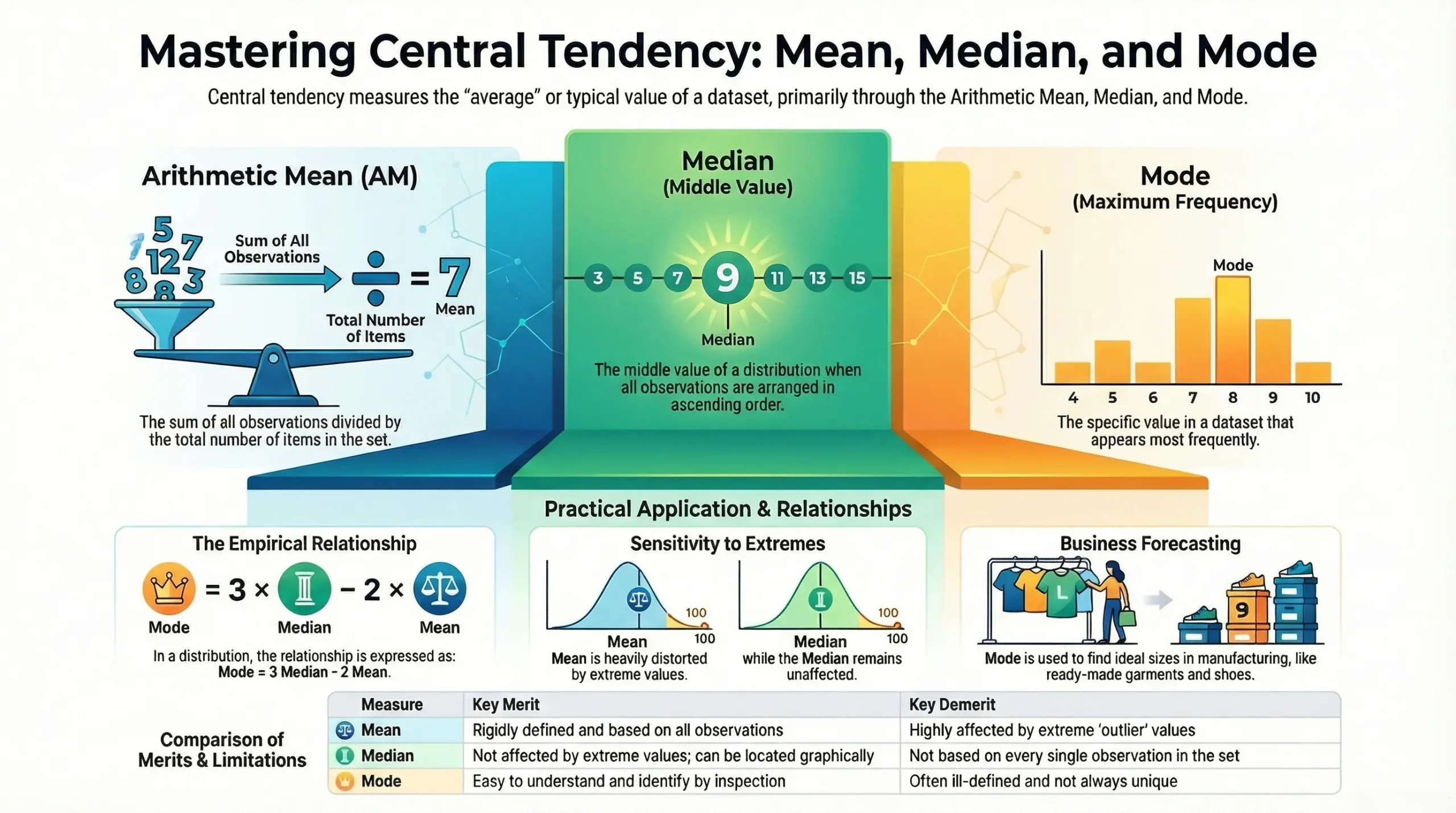
Measures of central tendency are statistical values that represent the center or typical value of a dataset. They provide a single value that summarizes the entire distribution. The three primary measures are:
- Arithmetic Mean (AM) or Simply Mean
- Median
- Mode
These measures help us understand the general trend of data and make meaningful comparisons between different datasets.
Arithmetic Mean
Arithmetic Mean is the sum of all observations divided by the total number of observations. It is the most commonly used measure of central tendency and represents the average value of a dataset.
Formula for Raw Data
For observations x₁, x₂, x₃, ..., xₙ:
Mean (x̄) = (x₁ + x₂ + x₃ + ... + xₙ) / n = Σxᵢ / n
Important Property:
n × x̄ = Σxᵢ
This means the product of mean and number of items equals the sum of observations.
Methods for Calculating Mean
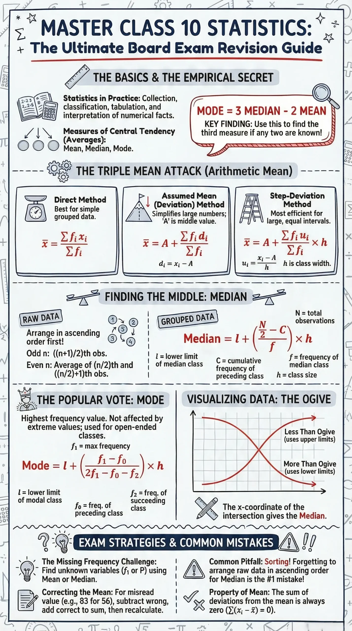
1. Direct Method (For Ungrouped Data)
Formula:
x̄ = Σfᵢxᵢ / Σfᵢ
Where:
- xᵢ = value of the variable
- fᵢ = frequency of xᵢ
2. Direct Method (For Grouped Data)
Steps:
- Find the mid-value (xᵢ) of each class interval
- Multiply each mid-value by its frequency (fᵢxᵢ)
- Sum all fᵢxᵢ values
- Divide by total frequency
Formula:
x̄ = Σfᵢxᵢ / Σfᵢ
3. Deviation Method (Assumed Mean Method)
This method simplifies calculations by using an assumed mean.
Formula:
x̄ = A + (Σfᵢdᵢ / Σfᵢ)
Where:
- A = Assumed mean (any value from the data, preferably the middle value)
- dᵢ = Deviation from assumed mean = (xᵢ - A)
- fᵢ = Frequency
4. Step-Deviation Method
This method further simplifies calculations when class intervals are uniform.
Formula:
x̄ = A + [(Σfᵢuᵢ / Σfᵢ) × h]
Where:
- A = Assumed mean
- uᵢ = (xᵢ - A) / h (coded deviation)
- h = Width of class interval
- fᵢ = Frequency
Properties of Arithmetic Mean
Sum of Deviations: The sum of deviations from the mean is always zero
- Σ(xᵢ - x̄) = 0
Addition Property: If a constant 'a' is added to each observation, the new mean = x̄ + a
Subtraction Property: If a constant 'a' is subtracted from each observation, the new mean = x̄ - a
Multiplication Property: If each observation is multiplied by constant 'a', the new mean = a × x̄
Division Property: If each observation is divided by constant 'a', the new mean = x̄ / a
Merits of Arithmetic Mean
- Rigidly Defined: Has a clear mathematical definition
- Easy to Calculate: Simple computational procedure
- Based on All Observations: Takes every data point into account
- Unique Value: Only one mean exists for a given dataset
- Least Affected by Sampling: Relatively stable across samples
- Algebraic Treatment: Can be used in further mathematical calculations
Demerits of Arithmetic Mean
- Cannot be Determined by Inspection: Requires calculation
- Not Suitable for Qualitative Data: Cannot measure qualities like beauty, honesty
- Affected by Missing Data: Cannot be computed if any observation is missing
- Sensitive to Extreme Values: Outliers can distort the mean significantly
- Misleading Without Context: May not represent the true nature of distribution
- Cannot Handle Open-Ended Classes: Classes like "below 10" or "above 90" create problems
- Not Suitable for Ratios: Cannot be used effectively for rates and proportions
Uses of Arithmetic Mean
- Academic Performance: Calculating average marks of students
- Statistical Estimates: Widely used in practical statistics
- Business Analysis: Finding profit per unit, output per machine, average monthly income and expenditure
- Economic Indicators: Computing average wages, prices, and production figures
Median
Median is the middle value of a distribution when data is arranged in ascending or descending order. It divides the dataset into two equal halves, where 50% of observations lie below it and 50% above it.
Calculation for Raw Data (Ungrouped Data)
Steps:
- Arrange the data in ascending order
- Count the number of observations (n)
Case 1: When n is odd
Median = Value of ((n+1)/2)ᵗʰ observation
Case 2: When n is even
Median = [Value of (n/2)ᵗʰ observation + Value of (n/2 + 1)ᵗʰ observation] / 2
Calculation for Grouped Data
Formula:
Median = ℓ + [(N/2 - C) / f] × h
Where:
- ℓ = Lower limit of the median class
- N = Total number of observations (Σfᵢ)
- C = Cumulative frequency of the class preceding the median class
- f = Frequency of the median class
- h = Size (width) of the median class
Identifying the Median Class
The median class is the class interval in which the (N/2)ᵗʰ item lies. To find it:
- Calculate N/2
- Prepare cumulative frequency column
- Identify the class whose cumulative frequency is greater than or equal to N/2
Merits of Median
- Rigidly Defined: Clear and unambiguous definition
- Easy to Understand: Simple concept to grasp
- Not Affected by Extreme Values: Outliers don't influence the median
- Graphical Representation: Can be located on a graph (ogive)
- Can be Determined by Inspection: Sometimes visible directly from data
- Handles Unequal Class Intervals: Works even when classes vary in size
Demerits of Median
- Inexact for Even Numbers: Not precisely defined when n is even
- Not Based on All Observations: Uses only the middle value(s)
- No Algebraic Treatment: Cannot be used in further mathematical operations
- Affected by Sampling Fluctuations: More variable than mean across samples
- Requires Arrangement: Data must be sorted first
Uses of Median
- Qualitative Characteristics: Ideal for data that can be ranked but not precisely measured (intelligence, socioeconomic status)
- Skewed Distributions: Better than mean when data has extreme values
- Economic Applications: Determining typical wages, distribution of wealth
- Housing and Real Estate: Finding typical property prices
Mode
Mode is the value that occurs most frequently in a dataset. It represents the most typical or common value in the distribution. A dataset may have:
- No mode (when all values occur equally)
- One mode (unimodal)
- Two modes (bimodal)
- Multiple modes (multimodal)
Mode for Ungrouped Data
Method: Inspection
- Count the frequency of each value
- The value with the highest frequency is the mode
Mode for Grouped Data (Continuous Frequency Distribution)
Formula:
Mode = ℓ + [(f₁ - f₀) / (2f₁ - f₀ - f₂)] × h
Where:
- ℓ = Lower limit of the modal class
- f₁ = Frequency of the modal class (highest frequency)
- f₀ = Frequency of the class preceding the modal class
- f₂ = Frequency of the class succeeding the modal class
- h = Width of the modal class
Identifying the Modal Class
The modal class is the class interval with the highest frequency.
Merits of Mode
- Easy to Understand: Simple concept
- Simple Calculation: Quick to compute
- Not Affected by Extreme Values: Outliers don't influence mode
- Can be Determined by Inspection: Often visible directly
- Handles Open-Ended Classes: Works even with classes like "above 100"
- Graphical Representation: Can be shown on graphs
Demerits of Mode
- Ill-Defined: Not always clearly defined; may not exist or may be multiple
- Not Based on All Observations: Only considers frequency
- No Algebraic Treatment: Cannot be used in mathematical operations
- Highly Affected by Sampling: Very variable across samples
- Indeterminate: May not give a definite value
Uses of Mode
- Business Forecasting: Predicting demand patterns
- Manufacturing: Determining ideal sizes for ready-made garments, shoes
- Quality Control: Identifying most common defect types
- Market Research: Finding most popular products or preferences
Empirical Relationship
For moderately skewed distributions:
Mode = 3 × Median - 2 × Mean
This formula provides an approximate mode value when direct calculation is difficult.
Cumulative Frequency Curves (Ogives)
An ogive (pronounced "oh-jive") is a cumulative frequency graph. It displays the cumulative frequency of classes in a frequency distribution and is used to determine median and other measures graphically.
Types of Ogives
1. Less Than Ogive
Construction:
- Convert frequency distribution to "less than" cumulative frequency
- Plot upper class limits on x-axis
- Plot cumulative frequencies on y-axis
- Join points with a smooth curve
Cumulative Frequency Format:
- Less than 10 → Cumulative frequency
- Less than 20 → Cumulative frequency
- Less than 30 → Cumulative frequency (and so on)
Characteristic: The curve rises from left to right (increasing curve)
2. More Than Ogive
Construction:
- Convert frequency distribution to "more than" cumulative frequency
- Plot lower class limits on x-axis
- Plot cumulative frequencies on y-axis
- Join points with a smooth curve
Cumulative Frequency Format:
- More than 0 → Cumulative frequency
- More than 10 → Cumulative frequency
- More than 20 → Cumulative frequency (and so on)
Characteristic: The curve falls from left to right (decreasing curve)
Finding Median from Ogive
Method:
- Draw both less than and more than ogives on the same graph
- Find N/2 on the y-axis (where N = total frequency)
- Draw a horizontal line from N/2 to meet the ogive
- From the intersection point, draw a perpendicular to the x-axis
- The value on x-axis is the median
Alternative (single ogive):
- For less than ogive: Locate N/2 on y-axis, draw horizontal to curve, then vertical to x-axis
- For more than ogive: Same process
Applications of Ogives
- Finding Median: Graphical determination
- Quartiles: Finding Q₁ (N/4) and Q₃ (3N/4)
- Percentiles: Any percentage point can be located
- Comparing Distributions: Visual comparison of two datasets
- Determining Number Below/Above: Finding how many observations fall below or above a certain value
Statistics Chapter 13 Class 10 Maths Solved Examples
Q. The mean of marks scored by 100 students was found to be 40. Later it was discovered that a score of 56 was misread as 83. Find the correct mean.
Solution:
Given: n = 100, x̄ = 40
Step 1: Find incorrect sum of observations
x̄ = Σxᵢ / n 40 = Σxᵢ / 100 Σxᵢ (incorrect) = 4000
Step 2: Correct the sum
Correct Σxᵢ = 4000 - 83 + 56 = 3973
Step 3: Calculate correct mean
Correct mean = 3973 / 100 = 39.73
The correct mean is 39.73
Q. Find the missing value P for the following distribution whose mean is 12.58
| x | 5 | 8 | 10 | 12 | P | 20 | 25 |
|---|---|---|---|---|---|---|---|
| f | 2 | 5 | 8 | 22 | 7 | 4 | 2 |
Solution:
Given: x̄ = 12.58
| xᵢ | fᵢ | fᵢxᵢ |
|---|---|---|
| 5 | 2 | 10 |
| 8 | 5 | 40 |
| 10 | 8 | 80 |
| 12 | 22 | 264 |
| P | 7 | 7P |
| 20 | 4 | 80 |
| 25 | 2 | 50 |
| Total | 50 | 524 + 7P |
Using the formula:
x̄ = Σfᵢxᵢ / Σfᵢ 12.58 = (524 + 7P) / 50 629 = 524 + 7P 7P = 105 P = 15
P = 15
Q. Find the mean for the following distribution:
| Marks | 10-20 | 20-30 | 30-40 | 40-50 | 50-60 | 60-70 | 70-80 |
|---|---|---|---|---|---|---|---|
| Frequency | 6 | 8 | 13 | 7 | 3 | 2 | 1 |
Solution:
| Marks | Mid-value (xᵢ) | Frequency (fᵢ) | fᵢxᵢ |
|---|---|---|---|
| 10-20 | 15 | 6 | 90 |
| 20-30 | 25 | 8 | 200 |
| 30-40 | 35 | 13 | 455 |
| 40-50 | 45 | 7 | 315 |
| 50-60 | 55 | 3 | 165 |
| 60-70 | 65 | 2 | 130 |
| 70-80 | 75 | 1 | 75 |
| Total | 40 | 1430 |
Mean = Σfᵢxᵢ / Σfᵢ = 1430 / 40 = 35.75
Mean = 35.75
Q. Find the mean for the following distribution using deviation method:
| xᵢ | 15 | 20 | 22 | 24 | 25 | 30 | 33 | 38 |
|---|---|---|---|---|---|---|---|---|
| fᵢ | 5 | 8 | 11 | 20 | 23 | 18 | 13 | 2 |
Solution:
Let Assumed Mean A = 25
| xᵢ | fᵢ | dᵢ = xᵢ - 25 | fᵢdᵢ |
|---|---|---|---|
| 15 | 5 | -10 | -50 |
| 20 | 8 | -5 | -40 |
| 22 | 11 | -3 | -33 |
| 24 | 20 | -1 | -20 |
| 25 | 23 | 0 | 0 |
| 30 | 18 | 5 | 90 |
| 33 | 13 | 8 | 104 |
| 38 | 2 | 13 | 26 |
| Total | 100 | 77 |
Mean = A + (Σfᵢdᵢ / Σfᵢ) Mean = 25 + (77 / 100) Mean = 25 + 0.77 = 25.77
Mean = 25.77
Q. Find the mean using step-deviation method:
| Class | 10-15 | 15-20 | 20-25 | 25-30 | 30-35 | 35-40 |
|---|---|---|---|---|---|---|
| Frequency | 5 | 6 | 8 | 12 | 6 | 3 |
Solution:
Let A = 27.5, h = 5
| Class | xᵢ | fᵢ | uᵢ = (xᵢ - 27.5)/5 | fᵢuᵢ |
|---|---|---|---|---|
| 10-15 | 12.5 | 5 | -3 | -15 |
| 15-20 | 17.5 | 6 | -2 | -12 |
| 20-25 | 22.5 | 8 | -1 | -8 |
| 25-30 | 27.5 | 12 | 0 | 0 |
| 30-35 | 32.5 | 6 | 1 | 6 |
| 35-40 | 37.5 | 3 | 2 | 6 |
| Total | 40 | -23 |
Mean = A + [(Σfᵢuᵢ / Σfᵢ) × h] Mean = 27.5 + [(-23 / 40) × 5] Mean = 27.5 + (-2.875) Mean = 24.625
Mean = 24.625
Q. The mean of the following frequency distribution is 62.8 and the sum of all frequencies is 50. Compute f₁ and f₂:
| Class | 0-20 | 20-40 | 40-60 | 60-80 | 80-100 | 100-120 |
|---|---|---|---|---|---|---|
| Frequency | 5 | f₁ | 10 | f₂ | 7 | 8 |
Solution:
Let A = 30, h = 20
| Class | xᵢ | fᵢ | uᵢ = (xᵢ-30)/20 | fᵢuᵢ |
|---|---|---|---|---|
| 0-20 | 10 | 5 | -1 | -5 |
| 20-40 | 30 | f₁ | 0 | 0 |
| 40-60 | 50 | 10 | 1 | 10 |
| 60-80 | 70 | f₂ | 2 | 2f₂ |
| 80-100 | 90 | 7 | 3 | 21 |
| 100-120 | 110 | 8 | 4 | 32 |
| Total | 30+f₁+f₂ | 58+2f₂ |
Given: Σfᵢ = 50
30 + f₁ + f₂ = 50 f₁ + f₂ = 20 ...(i)
Using mean formula:
62.8 = 30 + [(58 + 2f₂) / 50] × 20 62.8 = 30 + [(58 + 2f₂) × 2/5] 32.8 = [(58 + 2f₂) × 2/5] 164 = 116 + 4f₂ 4f₂ = 48 f₂ = 12
From equation (i):
f₁ + 12 = 20 f₁ = 8
f₁ = 8, f₂ = 12
Q. Find the mean marks from the following data:
| Marks | No. of Students |
|---|---|
| Below 10 | 5 |
| Below 20 | 9 |
| Below 30 | 17 |
| Below 40 | 29 |
| Below 50 | 45 |
| Below 60 | 60 |
| Below 70 | 70 |
| Below 80 | 78 |
| Below 90 | 83 |
| Below 100 | 85 |
Solution:
First, convert to grouped frequency:
| Marks | xᵢ | fᵢ | uᵢ (A=45, h=10) | fᵢuᵢ |
|---|---|---|---|---|
| 0-10 | 5 | 5 | -4 | -20 |
| 10-20 | 15 | 4 | -3 | -12 |
| 20-30 | 25 | 8 | -2 | -16 |
| 30-40 | 35 | 12 | -1 | -12 |
| 40-50 | 45 | 16 | 0 | 0 |
| 50-60 | 55 | 15 | 1 | 15 |
| 60-70 | 65 | 10 | 2 | 20 |
| 70-80 | 75 | 8 | 3 | 24 |
| 80-90 | 85 | 5 | 4 | 20 |
| 90-100 | 95 | 2 | 5 | 10 |
| Total | 85 | 29 |
Mean = A + [(Σfᵢuᵢ / Σfᵢ) × h] Mean = 45 + [(29 / 85) × 10] Mean = 45 + 3.41 = 48.41
Mean marks = 48.41
Q. Find the median of the following data representing lives (in hours) of 15 aircraft engine components:
715, 724, 725, 710, 729, 745, 649, 699, 696, 712, 734, 728, 716, 705, 719
Solution:
Step 1: Arrange in ascending order
649, 696, 699, 705, 710, 712, 715, 716, 719, 724, 725, 728, 729, 734, 745
Step 2: N = 15 (odd)
Median = Value of ((N+1)/2)ᵗʰ observation Median = Value of ((15+1)/2)ᵗʰ observation Median = Value of 8ᵗʰ observation Median = 716
Median = 716 hours
Q. Find the median wage of workers:
| Daily wages (Rs.) | 125 | 130 | 135 | 140 | 145 | 150 | 160 | 180 |
|---|---|---|---|---|---|---|---|---|
| No. of workers | 6 | 20 | 24 | 28 | 15 | 4 | 2 | 1 |
Solution:
| Wages | Workers | Cumulative Frequency |
|---|---|---|
| 125 | 6 | 6 |
| 130 | 20 | 26 |
| 135 | 24 | 50 |
| 140 | 28 | 78 |
| 145 | 15 | 93 |
| 150 | 4 | 97 |
| 160 | 2 | 99 |
| 180 | 1 | 100 |
N = 100 (even)
Median = [50ᵗʰ observation + 51ˢᵗ observation] / 2
From cumulative frequency, both 50ᵗʰ and 51ˢᵗ observations lie in:
- 50ᵗʰ observation = 135
- 51ˢᵗ observation = 140
Median = (135 + 140) / 2 = 137.50
Median wage = Rs. 137.50
Q. Calculate the median:
| Class | 0-10 | 10-20 | 20-30 | 30-40 | 40-50 | 50-60 |
|---|---|---|---|---|---|---|
| Frequency | 5 | 10 | 20 | 7 | 8 | 5 |
Solution:
| Class | f | c.f. |
|---|---|---|
| 0-10 | 5 | 5 |
| 10-20 | 10 | 15 |
| 20-30 | 20 | 35 |
| 30-40 | 7 | 42 |
| 40-50 | 8 | 50 |
| 50-60 | 5 | 55 |
N = 55, N/2 = 27.5
The 27.5ᵗʰ observation lies in class 20-30 (c.f. = 35)
Median class: 20-30
- ℓ = 20
- f = 20
- C = 15
- h = 10
Median = ℓ + [(N/2 - C) / f] × h Median = 20 + [(27.5 - 15) / 20] × 10 Median = 20 + (12.5 / 20) × 10 Median = 20 + 6.25 = 26.25
Median = 26.25
Q. The median of the following distribution is 46. Find f₁ and f₂:
| Variable | 10-20 | 20-30 | 30-40 | 40-50 | 50-60 | 60-70 | 70-80 | Total |
|---|---|---|---|---|---|---|---|---|
| Frequency | 12 | 30 | f₁ | 65 | f₂ | 25 | 18 | 229 |
Solution:
Total frequency equation:
12 + 30 + f₁ + 65 + f₂ + 25 + 18 = 229 150 + f₁ + f₂ = 229 f₁ + f₂ = 79 ...(i)
Median = 46 lies in class 40-50 (modal class has highest frequency 65)
| Class | Frequency | C.F |
|---|---|---|
| 10-20 | 12 | 12 |
| 20-30 | 30 | 42 |
| 30-40 | f₁ | 42 + f₁ |
| 40-50 | 65 | 107 + f₁ |
| 50-60 | f₂ | 107 + f₁ + f₂ |
For median class 40-50:
- ℓ = 40, h = 10, f = 65, C = 42 + f₁, N = 229
Median = ℓ + [(N/2 - C) / f] × h 46 = 40 + [(229/2 - (42 + f₁)) / 65] × 10 46 = 40 + [(114.5 - 42 - f₁) / 65] × 10 6 = [(72.5 - f₁) / 65] × 10 6 × 65 = (72.5 - f₁) × 10 390 = 725 - 10f₁ 10f₁ = 335 f₁ = 33.5 ≈ 34
From equation (i):
34 + f₂ = 79 f₂ = 45
f₁ = 34, f₂ = 45
Q. Find the mode:
25, 16, 19, 48, 19, 20, 34, 15, 19, 20, 21, 24, 19, 16, 22, 16, 18, 20, 16, 19
Solution:
Frequency table:
| Value | 15 | 16 | 18 | 19 | 20 | 21 | 22 | 24 | 25 | 34 | 48 |
|---|---|---|---|---|---|---|---|---|---|---|---|
| Frequency | 1 | 4 | 1 | 5 | 3 | 1 | 1 | 1 | 1 | 1 | 1 |
The value 19 has the maximum frequency of 5.
Mode = 19
Q. Find the mode:
| Age (Years) | 5-14 | 15-24 | 25-34 | 35-44 | 45-54 | 55-64 |
|---|---|---|---|---|---|---|
| No. of Cases | 6 | 11 | 21 | 23 | 14 | 5 |
Solution:
Convert to inclusive form:
| Age | 4.5-14.5 | 14.5-24.5 | 24.5-34.5 | 34.5-44.5 | 44.5-54.5 | 54.5-64.5 |
|---|---|---|---|---|---|---|
| Cases | 6 | 11 | 21 | 23 | 14 | 5 |
Modal class: 34.5-44.5 (highest frequency = 23)
- ℓ = 34.5
- f₁ = 23
- f₀ = 21
- f₂ = 14
- h = 10
Mode = ℓ + [(f₁ - f₀) / (2f₁ - f₀ - f₂)] × h Mode = 34.5 + [(23 - 21) / (46 - 21 - 14)] × 10 Mode = 34.5 + [2 / 11] × 10 Mode = 34.5 + 1.818 Mode = 36.32
Mode = 36.32
Q. Find the mode:
| Daily Wages | 31-36 | 37-42 | 43-48 | 49-54 | 55-60 | 61-66 |
|---|---|---|---|---|---|---|
| No. of workers | 6 | 12 | 20 | 15 | 9 | 4 |
Solution:
Convert to continuous classes (subtract 0.5 from lower limit, add 0.5 to upper limit):
| Wages | 30.5-36.5 | 36.5-42.5 | 42.5-48.5 | 48.5-54.5 | 54.5-60.5 | 60.5-66.5 |
|---|---|---|---|---|---|---|
| Workers | 6 | 12 | 20 | 15 | 9 | 4 |
Modal class: 42.5-48.5 (highest frequency = 20)
- ℓ = 42.5
- f₁ = 20
- f₀ = 12
- f₂ = 15
- h = 6
Mode = ℓ + [(f₁ - f₀) / (2f₁ - f₀ - f₂)] × h Mode = 42.5 + [(20 - 12) / (40 - 12 - 15)] × 6 Mode = 42.5 + [8 / 13] × 6 Mode = 42.5 + 3.69 Mode = 46.19
Mode = 46.19
Q. Draw less than ogive and find median:
| Marks | 0-10 | 10-20 | 20-30 | 30-40 | 40-50 | 50-60 |
|---|---|---|---|---|---|---|
| Students | 7 | 10 | 23 | 51 | 6 | 3 |
Solution:
Cumulative frequency table:
| Marks | No. of Students |
|---|---|
| Less than 10 | 7 |
| Less than 20 | 17 |
| Less than 30 | 40 |
| Less than 40 | 91 |
| Less than 50 | 97 |
| Less than 60 | 100 |
Steps to draw ogive:
- Plot upper class limits on x-axis (10, 20, 30, 40, 50, 60)
- Plot cumulative frequencies on y-axis
- Join points with smooth curve
To find median:
- N = 100, N/2 = 50
- Draw horizontal line from y = 50 to curve
- From intersection, draw perpendicular to x-axis
- Reading gives median ≈ 34
Median = 34 marks (graphically)
Q. Draw both less than and more than ogives for the medical entrance exam data:
| Marks | 400-450 | 450-500 | 500-550 | 550-600 | 600-650 | 650-700 | 700-750 | 750-800 |
|---|---|---|---|---|---|---|---|---|
| Examinees | 30 | 45 | 60 | 52 | 54 | 67 | 45 | 47 |
Solution:
Less Than Ogive:
| Marks | Cumulative Frequency |
|---|---|
| Less than 450 | 30 |
| Less than 500 | 75 |
| Less than 550 | 135 |
| Less than 600 | 187 |
| Less than 650 | 241 |
| Less than 700 | 308 |
| Less than 750 | 353 |
| Less than 800 | 400 |
More Than Ogive:
| Marks | Cumulative Frequency |
|---|---|
| 400 and more | 400 |
| 450 and more | 370 |
| 500 and more | 325 |
| 550 and more | 265 |
| 600 and more | 213 |
| 650 and more | 159 |
| 700 and more | 92 |
| 750 and more | 47 |
The intersection point of both ogives gives the median.
Finding specific values:
- Examinees with marks < 625: Draw vertical from x = 625, approximately 220
- Examinees with marks ≥ 625: 400 - 220 = 180
Q. The mean of 5 observations is 20. If 10 is added to each observation, what is the new mean?
Solution:
Original mean = 20
Using property: If constant 'a' is added to each observation, new mean = x̄ + a
New mean = 20 + 10 = 30
New mean = 30
Q. The mean salary of 50 employees is ₹25,000. If each salary is increased by 20%, what is the new mean salary?
Solution:
Original mean = ₹25,000 Increase = 20% = multiplying by 1.20
Using property: If each observation is multiplied by 'a', new mean = a × x̄
New mean = 1.20 × 25,000 = ₹30,000
New mean salary = ₹30,000
Q. For a moderately asymmetrical distribution, mean = 30 and median = 28. Find the mode.
Solution:
Using empirical formula:
Mode = 3 × Median - 2 × Mean Mode = 3 × 28 - 2 × 30 Mode = 84 - 60 Mode = 24
Mode = 24
Q. The mean marks of 40 students in Section A is 65, and the mean marks of 60 students in Section B is 70. Find the combined mean of all 100 students.
Solution:
For Section A:
- n₁ = 40, x̄₁ = 65
- Sum = 40 × 65 = 2600
For Section B:
- n₂ = 60, x̄₂ = 70
- Sum = 60 × 70 = 4200
Combined mean:
x̄ = (n₁x̄₁ + n₂x̄₂) / (n₁ + n₂) x̄ = (2600 + 4200) / (40 + 60) x̄ = 6800 / 100 x̄ = 68
Combined mean = 68
Conclusion
Statistics provides powerful tools for understanding and analyzing data. Mastery of measures of central tendency mean, median, and mode is fundamental for Class 10 students and forms the foundation for advanced statistical concepts. Practice with diverse problems, understand when to use each measure, and develop proficiency in both computational and graphical methods.
This comprehensive guide covers all aspects of the Class 10 Statistics curriculum, providing clear explanations, step-by-step solutions, and practical applications. Regular practice of solved examples and understanding the underlying concepts will ensure success in examinations and build strong analytical skills for future studies.